Case Study
Tawfic
A. Obeida![]() , Yousef S. Al-Mehairi
, Yousef S. Al-Mehairi![]() and Karri Suryanarayana
and Karri Suryanarayana
![]()
Abu Dhabi Company for Onshore Oil Operations (ADCO), P.O. Box 270, Abu Dhabi, UAE.
Received: 17 January 2005
Accepted: 14 April 2005
Published: 06 August 2005
This article is available from: http://petroleumjournalsonline.com/journals/index.php/petrophysics/article/view/1/6
© 2005 Obeida et al; licensee Petroleum Journals Online.
This is an Open Access article distributed under the
terms of the Creative Commons Attribution License (http://creativecommons.org/licenses/by-nc-nd/2.0/),
which permits unrestricted use for non-commercial purposes, distribution, and
reproduction in any medium, provided the original work is properly cited.
Calculation of initial fluid saturations is a critical step in any 3D reservoir modeling studies. The initial water saturation (Swi) distribution will dictate the original oil in place (STOIP) estimation and will influence the subsequent steps in dynamic modeling (history match and predictions). Complex carbonate reservoirs always represent a quit a challenge to geologist and reservoir engineers to calculate the initial water saturation with limited or no SCAL data available. The proposed method in this study combines core data (permeability) from 32 cored wells with identifiable reservoir rock types (RRTs) and log data (porosity and Swi) to develop drainage log-derived capillary pressure (Pc) based on rock quality index (RQI) and then calculate J-function for each RRT which was used to calculate the initial water saturation in the reservoir.
The initialization results of the dynamic model indicate good Swi profile match between the calculated Swi and the log-Swi for 70 wells across the field. The calculation of STOIP indicates a good agreement (within 3% difference) between the geological 3D model (31 million cells fine scale) and the upscaled dynamic model (1 million cells). The proposed method can be used in any heterogeneous media to calculate initial fluid saturations.
Reservoir characterization is an essential part of building robust dynamic models for proper reservoir management and making reliable predictions. A good definition of reservoir rock types should relate somehow the geological facies to their petrophysical properties. However, this was not the case in this work there is an overlap of petrophysical properties between the different RRTs. It was difficult to differentiate between the Mercury injection capillary curves (MIPCs) for a given RRT based of porosity and/or permeability ranges. Besides, the Mercury displacing air in the MIPc measurements does not represent the correct displacement mechanism in the reservoir.
The objectives of this study were:
A dynamic model was constructed by upscaling a 3-D geological model, 31 million cells, of the Lower Cretaceous Carbonate buildup in one of ADCO's oil fields in UAE. The carbonate formation presented here is the most prolific and geologically complex oil reservoir. 17 Reservoir Rock Types (RRTs) were described based on facies, porosity and permeability. Log derived permeability based on a Neural Network (3), honoring the core permeability was used in the 3D geological model. 30 faults and an areal distribution of a dense RRT were incorporated into the model based on seismic data interpretation.
Different simulation grids were realized to preserve the geological heterogeneity and the RRTs after upscaling of the geological model and the dynamic model was optimized to minimize the run time. Due to lack of pre-depletion RFTs, the free water level (FWL) was estimated from early pressure data (BHCIPs) and water saturation log from key transition zone wells.
All the core and log data from the 32 cored wells were filtered according to RRTs in a table format using EXCEL spread sheet software (see Table 1). The oil and water densities were measured at reservoir temperature (PVT data). The interfacial tension (IFT) between oil and brine also measured and assuming a contact angle of zero degree.
The calculation procedure can be handled using EXCEL spread sheet for each RRT as following:
1. For each data point (per foot), calculate the height (H) above the free water level (FWL):
H = FWL - TVDss (1)
2. Calculate the capillary pressure (Pc) for each height:
![]() (2)
(2)
3. For each data point (per foot), calculate the rock quality index (RQI):
![]() (3)
(3)
4. Use the linear multi-regression method to calculate the regression coefficients a, b and c from equation 4.
![]() (4)
(4)
5. Check the quality of regression by plotting the right hand side (RHS) of equation 4 versus the LHS (see Figure 1). If a unit slope line is obtained with R2 (at least greater than 0.8) close to one, then the regression is good and the coefficients a, b and c can be used to calculate the log-derived Pc at a given RQI using equation 5.
![]() (5)
(5)
Equation 5 gives a family of Pc's for each RRT for various RQI's as shown in Figure 2. Since ECLIPSE simulator uses a table format to enter the saturation functions, it would be unsuitable to enter several saturation functions (depending on RQI rage) for each RRT. This problem can be overcome by using a J-function for each RRT. In order to calculate a J-function for each RRT a single value of RQI for each RRT is needed.
6. Simple statistical method was used to calculate the mean value of RQI for each RRT. A plot of relative frequency versus RQI for RRT17 is shown in Figure 3. The mean value of RQI is 0.1264. This value was used to calculate the J-function for RRT17 using the definition of J-function in equation 6 (K in mD, porosity in fraction and Pc in psi):
![]() (6)
(6)
Equation 3 can be expressed as following:
![]() (7)
(7)
Substituting equation 7 into 6 yields equation 8 which was used to calculate the J-function at the mean RQI for each RRT.
![]() (8)
(8)
7. Since each saturation table starts with a minimum Swi (irreducible Swi), a plot of RQI versus Swi-log was generated for each RRT to estimate Swir as shown in Figure 4. The J-function and the relative permeability curves both start at the same Swir value.
The J-function option in ECLIPSE simulator scales the capillary pressure function (calculated from input J-function) according to the rock porosity and permeability for each grid cell. Therefore, the calculated water saturation is a function of Pc (height) as well as rock property (porosity and permeability). For this reason, the J(Sw) works better than normal Pc(Sw) in complex carbonates during model initialization.
Evaluation of the above procedure was tested first using measured laboratory data from well A1. The capillary pressure was measured using two core plugs (RRT 1) in oil/brine system. The first plug was cored from reservoir Unit A (phi=0.262, K=12.5 mD, RQI=0.217) and the second plug from reservoir Unit B (phi=0.282, K= 6.1 mD, RQI=0.146). Figure 5 shows the measured Pc data (points) and the calculated Pc (lines). It indicates a good match between the measured data and the calculated Pc at Pc values lower than 50 psi (transition zone Pc which is more important to match), but not so good at the higher Pc values (90 psi). However, it is more important to match the log Swi from several wells to have a successful model initialization.
70 wells across the field at initial water saturation (not affected by injected water) were selected for Swi profile comparisons. Figure 6 shows the well location of selected wells. The field has 600+ wells of producers and peripheral water injectors. It has 40 years of production history form three different production horizons. The maximum reservoir thickness is about 150 meters (500 feet) of carbonate formation. Part of the reservoir contains dense-porous cycles where the dense RRT has higher Swi than the other porous RRTs. Figures 7 and 8 show the Swi comparisons between the log-Swi and the calculated Swi from the model. 90% of the Swi comparisons indicate a good match. The calculated original oil in place (STOIP) from the geological model and the dynamic model indicated a good agreement (within 3% difference) between the two models.
First the model was initialized using MIPCs and J-functions calculated from core plugs, the Swi match was not good partially in the transition zone area. Then we tried to generate a Pc curve for each RRT from log data (industry standard methods), but the averaging technique to pick a single Pc curve was not good enough due to data spreading. Finally, the model was initialized using the log-derived J-functions described by the proposed method and the results are good as shown in figures 7 and 8.
Figure 7 shows the Swi comparison for wells P1, P2, P3 and P4. Well P1 was not logged to TD as indicated by Swi log (black dots). The Swi match is good as indicated by model Swi (red line). The thin layers on the top of the reservoir represent the RRTs with lower reservoir quality (low K and higher Swi). Well P2 was logged to TD, the Swi match is good, lower part of the reservoir also has lower quality RRTs which are marked by higher Swi intervals. The model is underestimates the Swi in some thin layers at lower reservoir units. Well P3 located in northern part of the reservoir where a thick dense low quality RRT with higher Swi existed. The Swi comparison indicated an acceptable match but it is not good as other matches. Well P4 indicated a good match. Figure 8 showing the Swi match for wells P5, P6, P7 and P8. Well P5 indicated a good match except in the layer just on top of 8050 where the model is overestimates the Swi. Well P6 was not logged to TD and it indicated a good match. Well P7 indicated a good match except in some layers (at 7850 and 8000) the model overestimates the Swi. Well P8 indicated a good match.
The rest of the wells were checked and evaluated the Swi match indicated a good match in 90% of the wells, 7% of the wells indicate an acceptable match and only 3% have bad match which maybe improved by redefining the RRTs and/or modifying the log-derived permeability in the vicinity of these wells.
In conclusion, a robust method was developed to generate log-derived Pcs and J-functions and calculate the initial water saturation in a giant complex carbonate reservoir better than these industry standard methods. This method maybe utilized if a limited or no SCAL data is available. The limitation of the proposed method is its dependency on log-derived permeability data.
The authors would like to acknowledge Abu Dhabi for Onshore Oil Operations (ADCO) for the permission and support to publish this work.
1. Alger, R.P., Luffel, D.L. and Truman, R.B.,1989. New Unified Method of Integrating Core Capillary Pressure Data with Well logs, SPE Formation Evaluation, 16793, 145-152.
2. Amaefule J.O., Altunbay M., Djebbar T., Kersey D. and Keen D.K.,1993. Enhanced Reservoir Description: Using Core and Log Data to Identify Hydraulic (Flow) Units and Predict Permeability in Uncored Intervals/Wells. SPE 26436, 1-16.
3. Badarinadh, V., Suryanarayana K., Yousef F.Z., Sahouh K., Valle A.: "Log-Derived Permeability in a Heterogeneous Carbonate Reservoir of Middle East, Abu Dhabi, Using Artificial Neural Network," SPE 74345, IPCEM, Mexico, February, 2002.
4. Obeida T. A. and M. H. Jasser, 2004. Shuaiba Full Field Development Plan Options. ADCO internal report. Abu Dhabi, UAE.
Table 1:Example of spread sheet data format for RRT 1
|
Input Data From Logs |
Calculated Data |
Regression Data |
||||||||
|
Y |
X1 |
X2 |
||||||||
|
Well No. |
Depth TVDss |
Log-Phi |
Log-K (md) |
Log Swi |
RQI |
Height (Feet)
|
Pc (psi) |
RQI(1-Swi) |
RQI |
Ln(Pc) |
|
P1 |
|
|
|
|
|
|
|
|
|
|
|
|
- |
- |
- |
- |
- |
- |
- |
- |
- |
- |
|
|
- |
- |
- |
- |
- |
- |
- |
- |
- |
- |
|
P2 |
|
|
|
|
|
|
|
|
|
|
|
|
- |
- |
- |
- |
- |
- |
- |
- |
- |
- |
 |
Figure 1: LHS of
Eq.4 [a+bRQI+cLn(Pc)] versus RHS [RQI(1-Sw_log)]
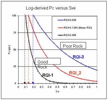
Figure 2:Ā Calculated Pcs at different RQIs versus Swi
 |
Figure 3: Frequency plot of RQI for RRT 17.
 |
Figure 4: RQI
versus Swi-log for RRT 17.
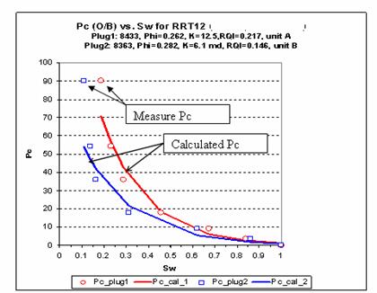
Figure 5: Pc versus Swi comparing measured and calculated Pc.
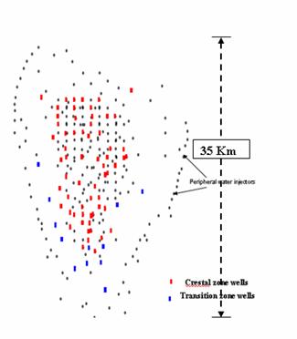
Figure 6: Location of wells used for Swi comparisons.
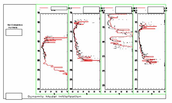
Figure 7: Swi comparison for wells P1, P2, P3 and P4.
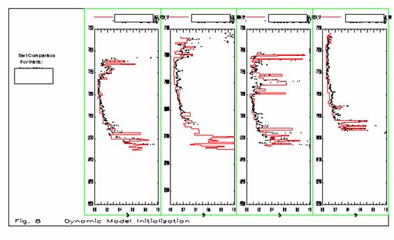
Figure 8: Swi comparison for wells P5, P6, P7 and P8.